The Finite Volume Method: A Comprehensive Introduction to Modern CFD

Why Computational Fluid Dynamics Matters

Computational Fluid Dynamics has revolutionized how engineers and scientists approach problems involving fluid flow and heat transfer. Where physical experiments once represented the only path to understanding complex flows, numerical simulation now offers a faster, more flexible, and often more economical alternative. Modern CFD enables researchers to peer inside flow domains where measurement probes cannot reach, to test thousands of design variations without building prototypes, and to answer 'what if' questions in hours rather than months.

The finite volume method stands as one of the most widely adopted approaches in this computational toolkit. Its popularity spans both academic research and industrial design workflows, from optimizing automobile aerodynamics to analyzing ventilation systems in buildings. This acceptance stems not from theoretical elegance alone, but from practical reliability: the method conserves physical quantities naturally and handles complex geometries gracefully.

From Physical Problem to Numerical Solution

Every CFD analysis begins with a physical question. Perhaps an aerospace engineer needs to reduce drag on an aircraft wing, or an automotive designer wants to minimize turbulence around a side mirror. The path from question to answer follows a structured progression that transforms continuous physics into discrete mathematics.

First comes the identification of governing equations—the partial differential equations that describe conservation of mass, momentum, and energy within the flow domain. These PDEs capture the physics exactly, but rarely yield analytical solutions for realistic geometries. The finite volume method bridges this gap by converting the continuous equations into a system of algebraic equations that computers can solve.

This transformation—from PDEs to linear algebra—constitutes the heart of numerical simulation. The finite volume method accomplishes it by dividing the spatial domain into discrete control volumes, then integrating the governing equations over each volume. What emerges is a linear system where each equation relates the solution at one point to values at neighboring points. Specialized linear solvers then extract the solution, which represents the original continuous field at discrete locations throughout the domain.

The Structure of a Finite Volume Course

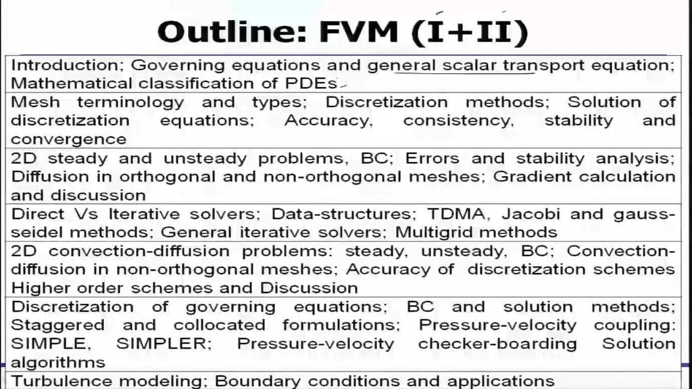
A comprehensive treatment of finite volume methods requires systematic development from first principles through advanced applications. The subject naturally divides into foundational concepts and advanced techniques, each building deliberately on what came before.

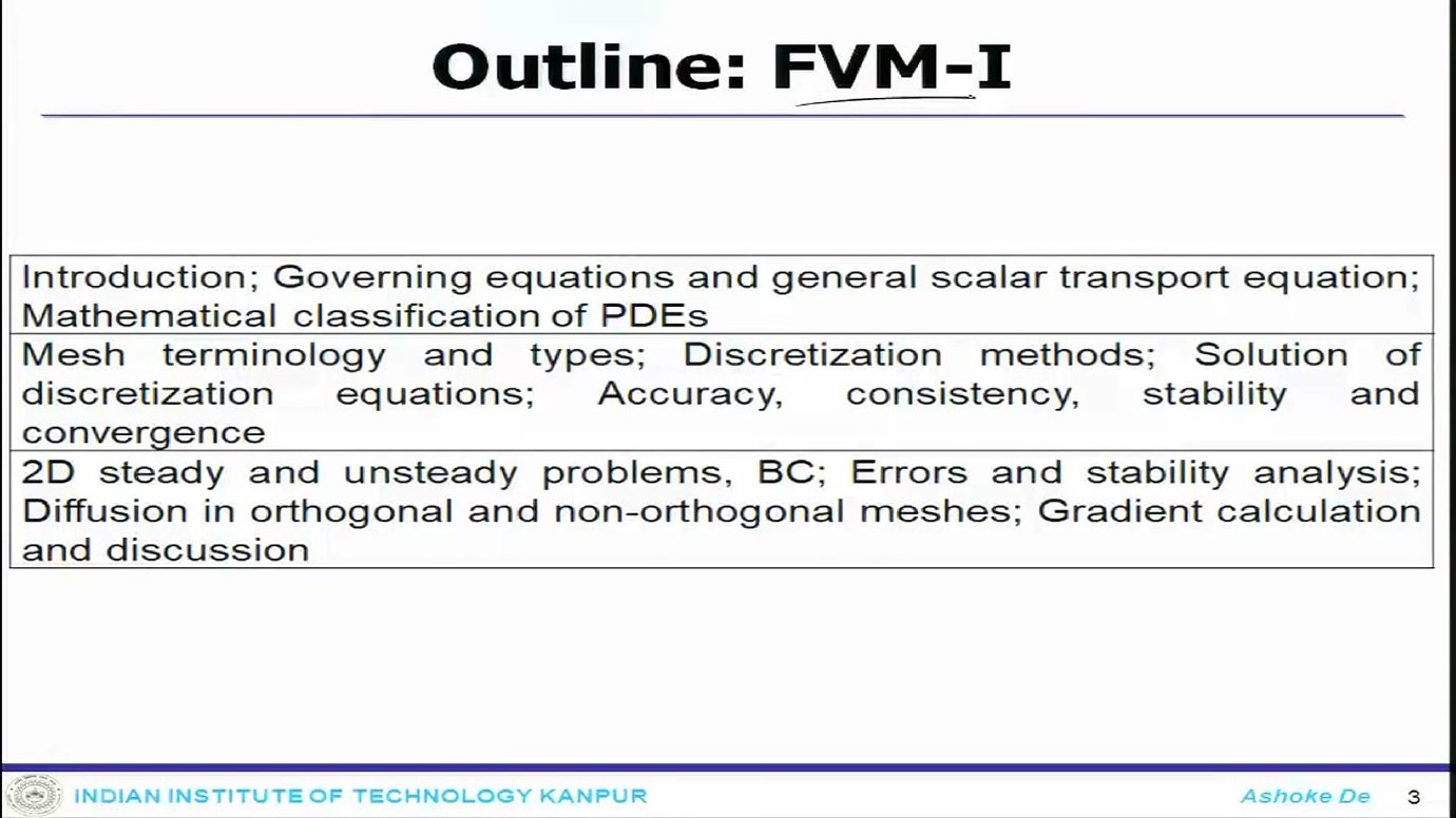
The foundational portion begins with governing equations—understanding what physical laws apply and how they manifest mathematically. This includes the general scalar transport equation and the classification of partial differential equations into elliptic, parabolic, and hyperbolic types. Each type exhibits distinct mathematical properties that influence how numerical methods must treat them.

Discretization follows as the next major topic. Here students learn mesh terminology, the types of computational grids available, and how to construct discrete equations that approximate the continuous originals. Critical concepts emerge: accuracy (how close does the discrete solution approach the continuous one?), consistency (does the discrete equation reduce to the continuous one as grid spacing vanishes?), stability (do errors grow or decay during computation?), and convergence (does the solution improve as the grid refines?).

With these tools in hand, the study turns to diffusion problems—scenarios where quantities spread due to gradients alone, without bulk motion. Two-dimensional steady and unsteady diffusion problems provide concrete contexts for exploring error analysis, stability requirements, and the special considerations that arise with orthogonal versus non-orthogonal grids. Gradient calculation methods receive particular attention, as accurate gradient computation proves essential for solution quality.

Linear Systems and Their Solution

Discretization produces linear systems—sometimes containing millions of equations for realistic problems. Solving these systems efficiently and accurately forms a discipline unto itself within computational methods.

Direct solvers approach the problem through matrix factorization techniques that guarantee a solution in a predictable number of operations. For small systems, direct methods prove both reliable and fast. But as problem size grows, their computational cost and memory requirements can become prohibitive.

Iterative solvers offer an alternative strategy. Rather than computing an exact solution through algebraic manipulation, these methods start with a guess and refine it through successive approximations. When properly designed, iterative methods converge to acceptable accuracy far faster than direct methods for large sparse systems—precisely the type that arises in finite volume discretization.

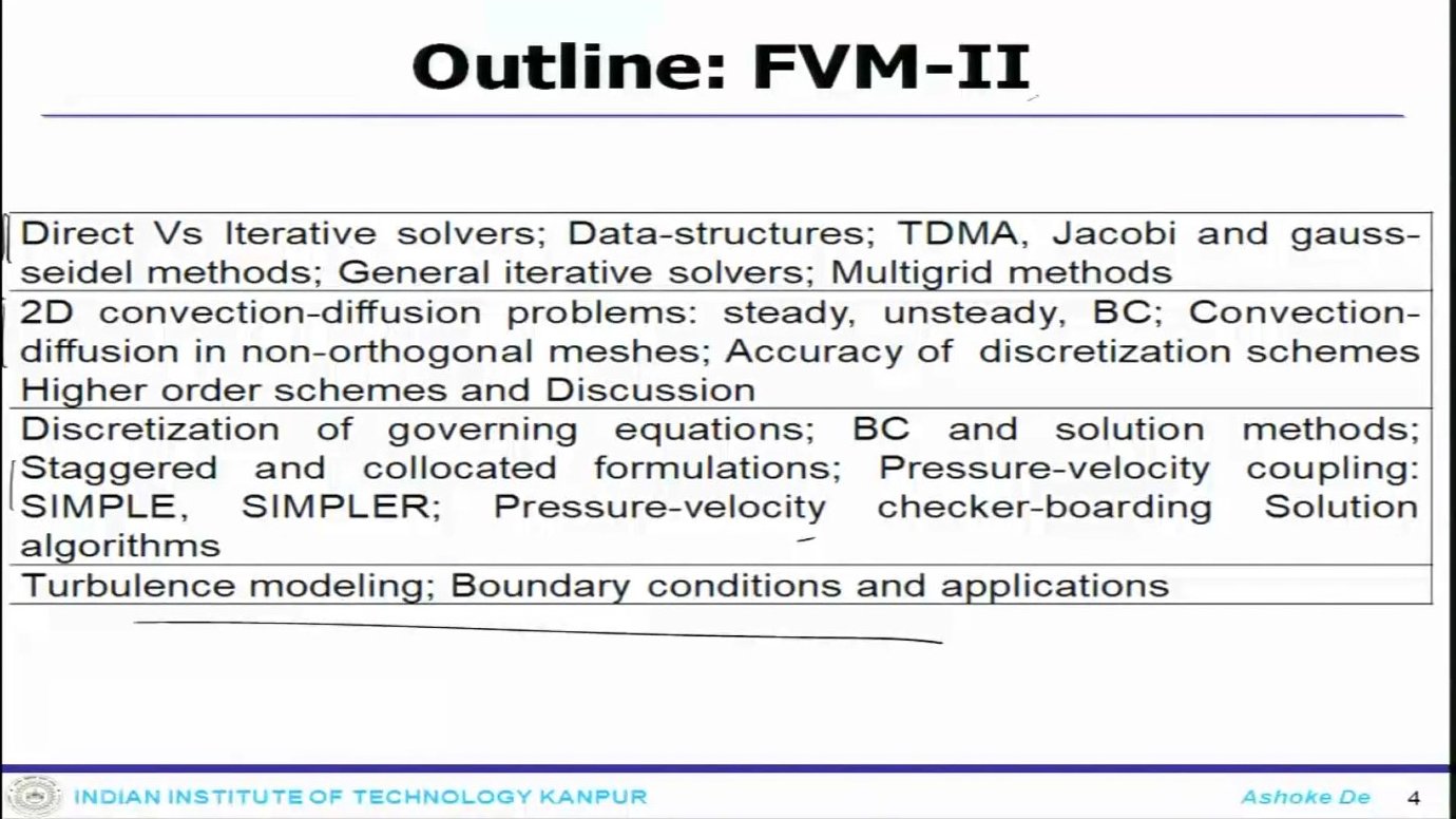
The study of linear solvers encompasses tridiagonal matrix algorithms (efficient for one-dimensional problems), Jacobi and Gauss-Seidel iterations (simple but sometimes slow), conjugate gradient methods (powerful for symmetric systems), and multigrid techniques (which accelerate convergence by solving on multiple grid resolutions simultaneously). Each approach carries distinct advantages for particular problem structures.

Convection-Diffusion Problems

Many realistic flows involve both diffusion (spreading due to gradients) and convection (transport by bulk fluid motion). The combination introduces new challenges that pure diffusion problems avoid.

When convection dominates diffusion—common in many engineering flows—numerical solutions can exhibit non-physical oscillations unless the discretization scheme incorporates special consideration for the flow direction. First-order upwind schemes eliminate oscillations by accounting for flow direction, but introduce numerical diffusion that smears sharp gradients. Higher-order schemes reduce this artificial diffusion while maintaining stability, but require more sophisticated implementation.

Boundary condition implementation becomes more nuanced with convection present. Inlet boundaries must specify both transported quantities and their fluxes. Outlet boundaries should allow disturbances to exit without reflecting back into the domain. Solid walls require no-slip conditions for velocity. Each boundary type demands careful numerical treatment to avoid corrupting the interior solution.

The distinction between orthogonal and non-orthogonal meshes gains importance in convection-diffusion problems. Orthogonal grids—where coordinate lines meet at right angles—simplify certain gradient calculations and generally produce more accurate solutions. Non-orthogonal grids offer geometric flexibility essential for complex geometries, but require additional correction terms to maintain accuracy. Understanding this trade-off guides mesh generation choices.

Fluid Flow and the Navier-Stokes Equations

The Navier-Stokes equations represent the pinnacle of classical fluid mechanics—a coupled system of nonlinear PDEs describing conservation of mass and momentum. Numerical solution of these equations presents challenges absent in simpler transport problems.

The pressure field introduces particular difficulty. Unlike velocity or temperature, which can often be specified at boundaries, pressure rarely appears in boundary conditions directly. Instead, pressure adjusts itself to ensure mass conservation (the continuity equation) while satisfying momentum conservation (the momentum equations). This coupling between pressure and velocity requires specialized solution algorithms.

Pressure-velocity coupling methods form a major topic in CFD. The SIMPLE algorithm (Semi-Implicit Method for Pressure-Linked Equations) and its variants SIMPLER and SIMPLEC represent one family of approaches. These methods iterate between solving momentum equations with a guessed pressure field, then correcting the pressure to satisfy continuity. Alternative formulations use artificial compressibility or solve all equations simultaneously, each approach carrying distinct computational costs and convergence properties.

Working in primitive variables—directly solving for pressure, velocity, and density—proves more intuitive and efficient than alternative formulations for most engineering problems. This choice simplifies boundary condition implementation and provides direct access to the quantities engineers care about. The resulting discretized equations preserve physical conservation laws, a key advantage of the finite volume approach.

Advanced Topics and Practical Applications

Beyond the fundamental solution techniques, several advanced topics extend the finite volume method's applicability to realistic engineering problems.

Turbulence modeling addresses the fact that most engineering flows operate at high Reynolds numbers where turbulent fluctuations dominate momentum and energy transport. Direct numerical simulation of all turbulent scales remains computationally intractable for most applications. Instead, turbulence models provide averaged equations with additional terms representing turbulent effects. The k-epsilon and k-omega models exemplify two-equation closures that balance accuracy against computational cost.

Boundary condition implementation for turbulence models requires care. Wall functions provide one approach, replacing direct resolution of the viscous sublayer with empirical correlations. Low-Reynolds-number formulations offer an alternative, extending the model validity to the wall but demanding finer grids. The choice impacts both solution accuracy and computational expense.

Moving beyond steady-state solutions to time-accurate unsteady simulations introduces temporal discretization considerations. Implicit methods allow larger time steps by solving coupled spatial-temporal systems, while explicit methods step forward in time using only known values but restrict step size for stability. The choice depends on whether the application demands resolving fast transients or merely reaching a steady state efficiently.

Learning Path and Prerequisites

Mastering finite volume methods requires progressive skill building. The subject divides naturally into two sequential courses, each building essential capabilities.

The first course establishes fundamentals: governing equations, discretization principles, mesh concepts, and solution of diffusion problems. Students completing this foundation should understand how continuous physics transforms into discrete algebra and how to solve the resulting systems. Hands-on programming—implementing simple one- and two-dimensional solvers—cements these concepts far better than passive study.

The second course assumes this foundation and builds toward complete flow solvers. Linear solver theory deepens, convection receives full treatment, and the Navier-Stokes equations finally yield to systematic solution procedures. Advanced topics like turbulence modeling and complex boundary conditions round out the treatment. By course end, students should possess the knowledge to tackle realistic engineering problems, either by writing custom codes or by using commercial software with genuine understanding of the underlying numerics.