Lift Curve Slope: From Airfoil Theory to Wing Design

The Finite Wing Effect on Lift Generation

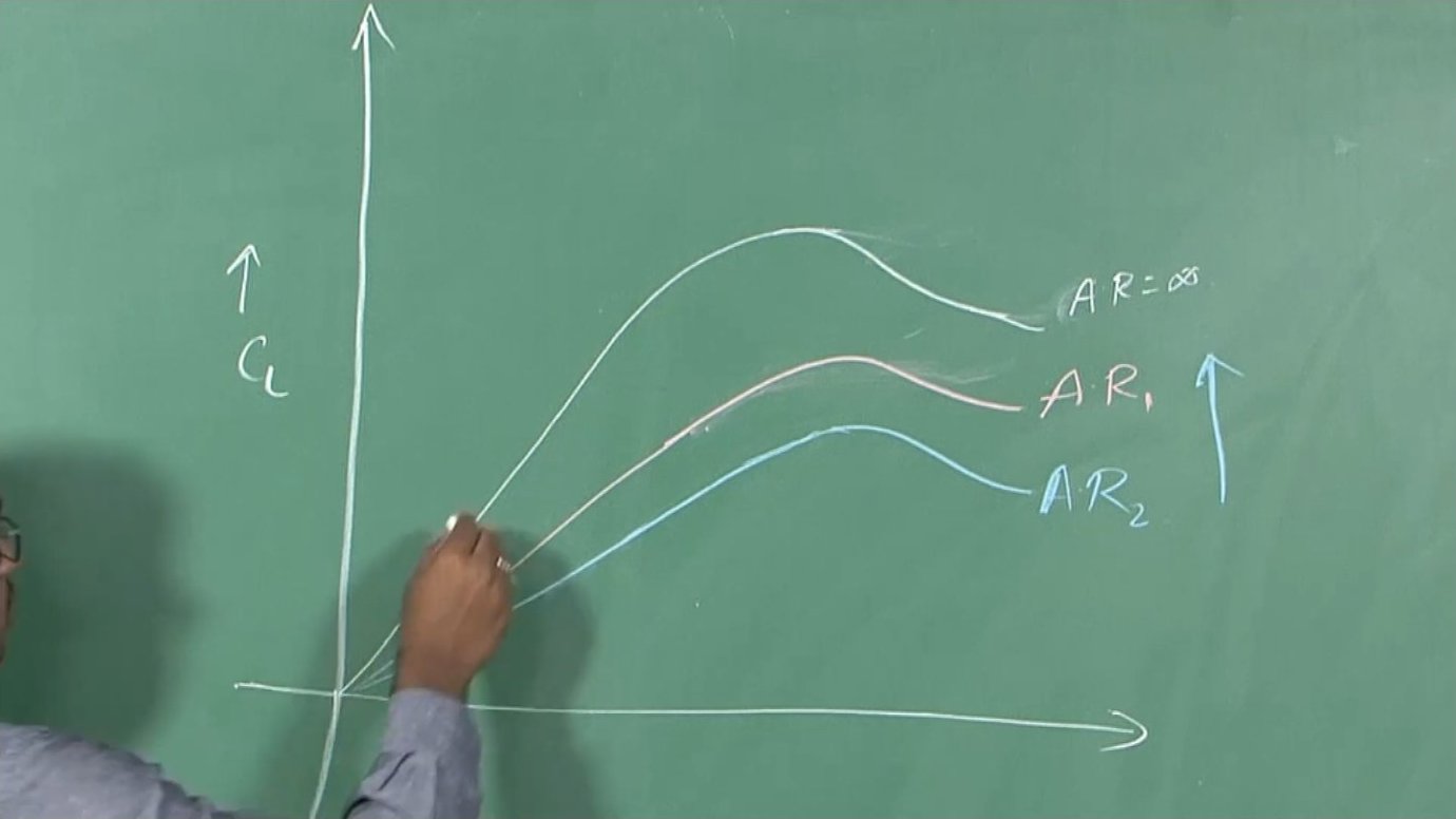
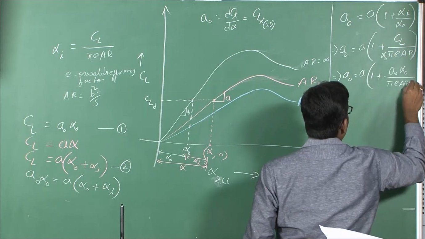
An airfoil operating in a theoretical two-dimensional environment generates lift differently than a finite wing. The crucial distinction lies in induced effects: real wings have tips where high-pressure air from below curls around to the low-pressure upper surface, creating trailing vortices. These vortices induce a downward velocity component—downwash—that effectively rotates the local flow direction at the wing, requiring a higher geometric angle of attack to produce the same lift coefficient.

The lift curve slope—the rate at which lift coefficient increases with angle of attack—decreases as aspect ratio decreases. For an infinite aspect ratio (the theoretical 2D airfoil case), no induced effects exist. As aspect ratio falls, the wing must operate at increasingly higher angles of attack to achieve the same lift coefficient. This fundamental relationship governs how engineers translate wind tunnel airfoil data into predictions for actual finite wings.

The induced angle of attack quantifies this penalty. It represents the additional angle required beyond what the airfoil alone would need. According to classical lifting-line theory, this induced angle equals CL/(π·e·AR), where CL is the lift coefficient, e is the Oswald efficiency factor (accounting for non-ideal span loading), and AR is the aspect ratio (span squared divided by planform area).

Deriving the Wing-Airfoil Relationship

Consider an airfoil and a wing built from that airfoil, both trimmed to produce identical lift coefficients. The airfoil achieves this at angle α₀, while the wing requires α₀ + αᵢ, where αᵢ is the induced angle. Since both generate the same CL, their lift equations must balance: a₀·α₀ = a·(α₀ + αᵢ), where a₀ is the 2D lift curve slope and a is the 3D slope.

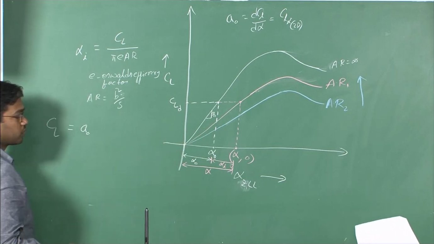
Rearranging this equality and substituting the expression for induced angle yields the fundamental relationship between 2D and 3D lift curve slopes. The 3D slope equals the 2D slope divided by (1 + a₀/(π·e·AR)). This denominator—always greater than unity for finite wings—explains why the wing's lift curve is always shallower than the airfoil's. The relationship reveals that lower aspect ratios produce more dramatic reductions in slope, while higher aspect ratios approach the 2D ideal.

Reading Airfoil Performance Data

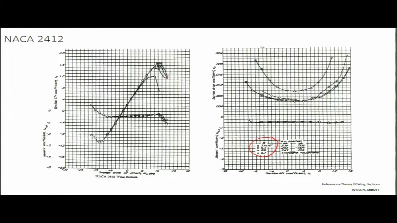
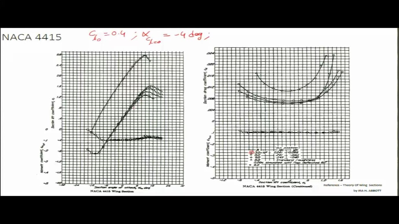
Standard airfoil data, compiled from wind tunnel testing, presents lift coefficient versus angle of attack curves for various Reynolds numbers. Extracting design parameters from these plots requires systematic reading. The zero-lift angle—where the curve crosses the horizontal axis—defines the reference from which other measurements proceed. For cambered airfoils, this occurs at negative angles because the camber generates lift even at zero geometric angle.

The lift coefficient at zero angle of attack, Cl₀, indicates the camber's contribution—symmetrical airfoils have Cl₀ = 0, while cambered sections show positive values. The lift curve slope emerges from selecting two points in the linear region and computing the rise over run, converting the angle increment to radians. The stall angle marks where the curve peaks, and the corresponding maximum lift coefficient defines the upper limit of usable angle of attack.

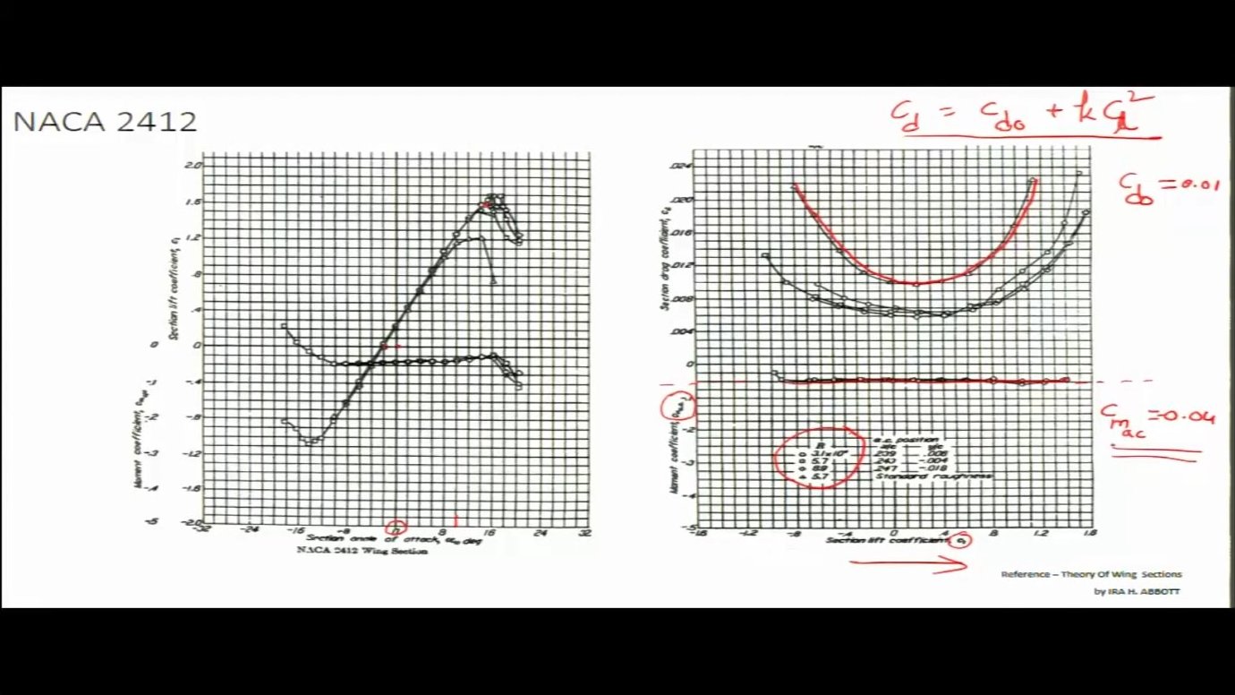
Drag polars—plots of drag coefficient versus lift coefficient—reveal the profile drag at zero lift (Cd₀) and confirm the parabolic relationship CD = Cd₀ + k·CL². The induced drag factor k relates to aspect ratio through k = 1/(π·e·AR). Moment coefficient plots, when nearly constant with angle of attack, identify the aerodynamic center location—typically at the quarter-chord for subsonic airfoils.

NACA Four-Digit and Five-Digit Series

The NACA four-digit series encodes geometry in its designation. For NACA 2412, the first digit specifies maximum camber as a percentage of chord (2%), the second gives the location of maximum camber in tenths of chord (at 0.4c), and the final two digits represent maximum thickness as a percentage of chord (12%). This systematic nomenclature allows engineers to select airfoils based on required characteristics without consulting detailed coordinate tables.

Five-digit series airfoils, such as NACA 23012, use a different coding. Here the first digit approximates the design lift coefficient in tenths (Cl ≈ 0.2), the next two specify the location of maximum camber in percent chord (at 15% chord for the '30'), and the final two again denote maximum thickness percentage. Both series exhibit similar characteristics: higher camber increases Cl₀ and shifts the zero-lift angle more negative, while greater thickness typically raises the maximum lift coefficient but increases drag.

Low-Drag Six-Series Airfoils

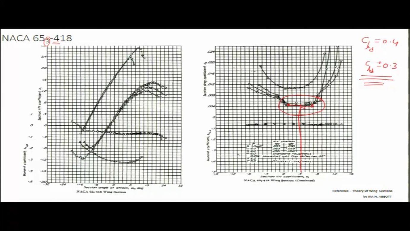
The NACA six-series represents a departure from earlier families, designed using theoretical pressure distributions rather than geometric construction. The defining feature is the drag bucket—a range of lift coefficients over which drag remains nearly constant and minimal. This occurs because the boundary layer remains laminar over a significant chord fraction when operating near the design lift coefficient.

For NACA 653-418, the designation reveals key design parameters. The '6' indicates the series, '5' represents the location of minimum pressure in tenths of chord (at 50% chord), the subscript '3' specifies the width of the low-drag range as three-tenths of Cl on either side of the design point, '4' gives the design lift coefficient in tenths (Cl = 0.4), and '18' represents maximum thickness percentage.

The drag bucket's practical value lies in cruise efficiency. An aircraft operating within this range experiences significantly lower drag than predicted by simple parabolic polars. However, outside the bucket—at lower or higher lift coefficients—drag rises sharply. Designers therefore select six-series airfoils when cruise conditions dominate mission requirements and can be tightly constrained.

Application: Wing Design from Airfoil Data

Consider designing a wing-alone UAV with 10-meter span and 11 m² area using the NACA 2412 airfoil. The Oswald efficiency factor is 0.75 and profile drag coefficient 0.02. From the airfoil data at Reynolds number 3 million, Cl₀ = 0.21 and the lift curve appears linear up to 8 degrees. At that angle, Cl ≈ 1.1. The slope calculation proceeds by selecting two points in the linear region and computing: Cl_α = (1.1 - 0.21) / (8° × π/180) = 6.374 per radian.

The aspect ratio equals (10)² / 11 = 9.09, yielding an induced drag factor k = 1/(π × 0.75 × 9.09) = 0.0466. Applying the transformation formula: CL_α = 6.374 / [1 + 6.374/(π × 0.75 × 9.09)] = 4.91 per radian. The wing's lift curve slope is thus 23% lower than the airfoil's, a direct consequence of the moderate aspect ratio.

A critical assumption links the two curves: the angle at which lift becomes zero remains identical for airfoil and wing. For NACA 2412, this occurs at -2 degrees. With this anchor point and the calculated slope, the wing's zero-angle lift coefficient follows: CL₀ = 4.91 × (-2° × π/180) = 0.172. The complete wing lift equation becomes CL = 0.172 + 4.91·α, enabling prediction of lift coefficient at any angle within the linear range.

At specific trim angles, both lift and drag emerge. At 3 degrees, CL = 0.429 and CD = 0.02 + 0.0466(0.429)² = 0.029. At 5 degrees, CL = 0.600 and CD = 0.037. At 7 degrees, CL = 0.772 and CD = 0.048. These values define the aircraft's performance map: for any required lift coefficient, the necessary angle of attack and resulting drag follow immediately.

Inverse Problem: Selecting an Airfoil

The inverse problem reverses the calculation: given a wing geometry and required trim condition, determine what airfoil characteristics are needed. Consider a triangular planform UAV with 1.5-meter span and 45-degree leading-edge sweep. The design lift coefficient is 0.334 at a 3-degree trim angle. What airfoil section lift curve slope is required?

The planform geometry determines area: for a triangle, A = (1/2) × base × height. The 45-degree sweep creates a right triangle with both legs equal to the semi-span (0.75 m), giving root chord 0.75 m and area 0.5625 m². Aspect ratio becomes (1.5)² / 0.5625 = 4.0. With the Oswald factor assumed as 0.75, the induced drag factor equals 1/(π × 0.75 × 4) = 0.106.

Assuming the zero-lift angle remains -2 degrees for both airfoil and wing, the wing's lift curve slope follows from the design point: CL_α = 0.334 / [3° - (-2°)] × (180/π) = 3.83 per radian. Inverting the transformation formula to solve for the required airfoil slope: Cl_α = CL_α / [1 - CL_α/(π·e·AR)] = 3.83 / [1 - 3.83/(π × 0.75 × 4)] = 6.45 per radian.

The airfoil's zero-angle lift coefficient emerges from the constraint that its zero-lift angle matches the wing's: Cl₀ = -Cl_α × α(Cl=0) = -6.45 × (-2° × π/180) = 0.225. An airfoil catalog search would now seek sections with Cl_α near 6.45 per radian and Cl₀ near 0.225—characteristics typical of moderately cambered four-digit NACA airfoils in the 2400 or 4400 series.

Performance Prediction from Integrated Data

A complete design example integrates geometry, airfoil selection, and operating conditions. A UAV with 2-meter span uses the NACA 653-418 airfoil, has a tip chord of 0.3 m and 31-degree leading-edge sweep, and requires CL = 0.4 in cruise. What trim angle of attack achieves this condition?

The trapezoidal planform's root chord follows from geometry: the semi-span (1 m) and sweep define the taper. Using tan(31°) = (CR - 0.3)/1 yields CR = 0.9 m. Area equals the average chord times span: A = 2 × (0.3 + 0.9)/2 = 1.2 m². Aspect ratio becomes (2)² / 1.2 = 3.33, another low-aspect-ratio configuration.

From the airfoil data at 3 million Reynolds number, Cl₀ = 0.3 at zero angle, and at 6 degrees, Cl = 0.9. The slope: Cl_α = (0.9 - 0.3)/(6° × π/180) = 5.73 per radian. The zero-lift angle reads as -2 degrees from the plot. Transforming to 3D: CL_α = 5.73 / [1 + 5.73/(π × 0.75 × 3.33)] = 3.32 per radian.

The wing's zero-angle lift coefficient: CL₀ = -3.32 × (-2° × π/180) = 0.116. To achieve CL = 0.4, the required trim angle follows from CL = CL₀ + CL_α × α: α = (0.4 - 0.116)/3.32 = 0.0857 radians, or 4.9 degrees. This moderate angle confirms the design operates well within the linear regime, with substantial margin below stall.

The Design Iteration Cycle

Aircraft design proceeds iteratively between airfoil selection, planform geometry, and performance requirements. Initial estimates of required lift coefficient—based on weight, cruise speed, and altitude—constrain airfoil choice. The selected airfoil's characteristics, combined with chosen aspect ratio and span, determine the achievable lift curve slope. This slope, in turn, dictates trim angles at various flight conditions.

If calculated trim angles fall outside acceptable ranges—too high, approaching stall, or too low, requiring excessive nose-down control deflection—the designer adjusts either the planform (changing aspect ratio or area) or the airfoil (selecting higher camber or different design lift coefficient). Drag considerations enter through the induced factor and profile drag, influencing power plant sizing and fuel requirements.

Modern computational tools automate these calculations, but the underlying relationships remain unchanged. Understanding how aspect ratio diminishes lift effectiveness, how camber sets the zero-angle coefficient, and how the drag polar governs efficiency allows engineers to make informed first-pass selections before expensive analysis or testing begins. The 2D-to-3D transformation serves as the conceptual foundation for every subsequent refinement.